A Junior Engineer's Guide to ClickHouse: The MergeTree Mental Model
ClickHouse on AWS: Self-Managed from First Principles · Part 1
ClickHouse stores logs well because of one table engine: MergeTree.
Almost everything else in this series builds on how MergeTree writes data, merges it in the background, and skips data with the ORDER BY key. Reference: MergeTree table engine. I run a log analytics platform on it. This post explains the storage model step by step, with the failure modes I have personally triggered. One running example carries the post: a warehouse that receives goods in sealed boxes. Each section notes where the picture stops matching the real mechanism.
Coming from Postgres? This post is the full walkthrough, but it assumes some comfort with storage concepts. If you want the gentler on-ramp first — the same warehouse model built from a five-year-old’s question, with a Postgres translator at every step (b-tree → sparse index, autovacuum → merges, MVCC → eventual consistency) — read Postgres Was a Filing Cabinet. ClickHouse Is a Warehouse first, then come back here for the operator’s depth: part explosions, TTL mechanics, and async-insert tuning.
Key takeaways
- Each INSERT becomes a part, and background merges compact many parts into fewer, larger ones. The system stays healthy only if merges keep up with insert rate.
- The ORDER BY key is the index. Every 8192 rows form a granule with recorded key ranges; queries skip whole granules.
- Columnar storage means a status-count query over a day of logs reads two columns, not whole rows.
- Never insert tiny batches. Past 1000 parts per partition, inserts get slowed; past 3000, they are rejected by default.
- Use SummingMergeTree and AggregatingMergeTree for rollup tables, not for raw log storage.
Columnar means you read what you asked for
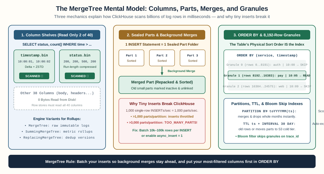
MergeTree stores each column in its own file, writes one sealed sorted part per INSERT that background workers compact, and uses a sparse ORDER BY index to skip 8,192-row granules.
Imagine a library that shelves books by attribute. All the titles stand together on one shelf. All the authors stand together on another shelf. To count books by subject, you open only the subject shelf. A column store works the same way: each shelf is one column file.
A row store like Postgres is different. It writes each log line as one contiguous row, like a library that binds each book’s title, author, and subject into one volume. To count subjects you must open every volume. That layout is fine for “fetch me user 42’s profile” but poor for aggregates over a billion rows. The analogy breaks down on one point: a real book is one object, but a table row is just 40 values. The point is only the arrangement — by attribute or by row.
SELECT status, count()
FROM events
WHERE timestamp >= now() - INTERVAL 1 DAY
GROUP BY status
This table might have 40 columns. The query reads two of them: timestamp and status. Everything else stays on disk.
COUNT by status, 40-column table:

Row store:     read all 40 columns of every scanned row
Column store:  read 2 of 40 files
Compression is the second benefit: sorted, similar values compress dramatically.
Parts and merges: the warehouse in the background
When you INSERT a batch of rows, ClickHouse writes a part: a self-contained directory holding that batch, sorted by the table’s ORDER BY key. Each INSERT makes exactly one part. No part is ever modified after creation.
Think of a warehouse receiving deliveries. Each delivery truck unloads one sealed box. The box is sorted inside before the tape goes on. The warehouse never opens a sealed box to edit it. In ClickHouse terms, the box is the part, and the truck is your INSERT statement.
Background merges continually fold smaller parts into larger ones, after the write, asynchronously. In the warehouse picture, a worker periodically repacks many small boxes into one bigger box. The worker never edits the contents, only the packaging. That is why inserts are fast: no sorting or index work happens at write time. But a query must read every matching part, and more parts means more files to open and slower queries. This tension between write speed and part count drives the insert strategy below.
The ORDER BY key is your index
ClickHouse has no traditional b-tree. The ORDER BY key in your CREATE TABLE is the index. It defines the sort order inside every part.
Think of a phone book sorted by last name. To find “Kumar” you do not read every page. You open the book directly at the K section. A sorted card index at a library works the same way. In ClickHouse terms, the ORDER BY key is the sort order of the card index, and the rows are the cards.
CREATE TABLE events
(
    timestamp    DateTime,
    service      LowCardinality(String),
    status       UInt16,
    ...
)
ENGINE = MergeTree
PARTITION BY (toYYYYMMDD(timestamp), toHour(timestamp))
ORDER BY (timestamp, service)
TTL toDateTime(timestamp + INTERVAL 30 DAY)
SETTINGS index_granularity = 8192
Note the ordering: timestamp first, service second. The second column only helps queries that also filter on timestamp. The set of leading sort columns a query filters on is called the prefix.
Inside a part, rows are grouped into granules of 8192 rows (index_granularity, the default). ClickHouse records each granule’s first row as the primary index entry and knows each granule’s min/max key range.
In the card-index picture, a granule is one drawer of the index. Each drawer has a label: “this drawer covers last names A through F.” A query for “Kumar” skips every drawer labeled G through Z without opening it. In ClickHouse terms, the drawer is a granule and the label is the recorded min/max key range. A query filtering timestamp >= '2026-11-05 00:00:00' never opens granules whose max timestamp is below that.
Part on disk, sorted by timestamp:
[granule 1][granule 2][granule 3] ...
  8192 rows  8192 rows
    ▲          ▲
    └── primary index: one entry per granule (sparse!)
This is a sparse index: one index entry per 8192 rows, not per row. It is tiny — a few kilobytes (KB) per million rows — and always in memory. It tells you which granules are worth opening, not where any single row is. The analogy breaks down on one point: a phone book points you to one name, but a sparse index points to a block of 8192 rows, which ClickHouse then scans. That keeps the index small enough to stay in memory.
Partitioning and time-to-live (TTL): scoping the work
PARTITION BY splits a table into disjoint chunks on disk — one directory per partition — and merging and dropping happen partition by partition. Reference: custom partitioning key.
Think of a filing room with one cabinet per day. A query about today opens only today’s cabinet. When a cabinet is no longer needed, you carry the whole cabinet out in one move. In ClickHouse terms, each cabinet is a partition, and DROP PARTITION is the one-move removal.
On the platform I run, every log table uses:
PARTITION BY (toYYYYMMDD(timestamp), toHour(timestamp))
That gives one partition per hour of fresh logs. Why hour and not day: DROP PARTITION of expired hours is instant, and each TTL merge has less work per step.
TTL deletes data on a schedule without manual cleanup:
TTL toDateTime(timestamp) + INTERVAL 30 DAY
Think of a rule that shreds paper older than 30 days. Nobody schedules the shredding; it is part of the filing rule itself. Every table keeps a 30-day TTL. Expired rows get dropped by background TTL merges, and whole expired partitions are dropped with a fast metadata operation. Without TTL, a log table grows until disk alarms fire. With TTL, retention is just another column expression.
Bloom filters for columns the primary index can’t help
The sparse primary index covers the ORDER BY key columns. Some columns are not in the sort key but are queried constantly, typically high-cardinality strings such as trace identifiers (IDs) and request IDs. For those we add a bloom filter: a probabilistic set that answers “definitely not in this granule” cheaply.
Put a quick checklist on the front of each card-index drawer: “this drawer contains no entries starting with G.” You read the label and skip the drawer without opening it. The checklist has one quirk: it can say “maybe” when the item is actually absent (a false yes), but it never says “no” when the item is present. In ClickHouse terms, the checklist is the bloom filter, the drawer is a granule, and a false “maybe” only means a few extra granules get opened.
INDEX idx_trace_id trace_id TYPE bloom_filter GRANULARITY 1
Those indexes run at a 0.01 (1%) false-positive rate. A 1% false positive is fine: the filter only adds extra granules to the read set, it never drops data.
Why logs fit this model
Log workloads have three properties that MergeTree was designed around:
- Append-only. Log lines never get updated after arrival. Parts are immutable, so there is no undo log and no write amplification from updates.
- Time-ordered. Arrival order matches sort order, so time-range queries can skip granules and TTL merges stay cheap.
- High, bursty insert rate. One part per INSERT means insert cost is flat regardless of batch size. The system absorbs bursts in merge queue depth, not in latency.
If you need row-level updates on arrival, MergeTree is the wrong tool. That is why the platform writes logs to a MergeTree table and keeps mutable metadata in Postgres.
The failure mode: “Too many parts”
Here is the mistake every new ClickHouse operator makes: inserting one row at a time, or in very small batches. At first it works. But each INSERT still makes a part.
Back to the warehouse. Suppose trucks deliver one tiny envelope every second. The box-combining worker falls behind, and the floor fills with unopened envelopes. Eventually the warehouse refuses new deliveries until the pile shrinks. That is exactly what ClickHouse does.
1 insert/second × 3600 = 3,600 parts/hour in that partition
Merges fold parts at some rate. If inserts outpace merges → part count grows.
Merge throughput scales with part count and central processing unit (CPU), but it is not infinite. When active parts per partition reaches parts_to_delay_insert (1000 by default), the server deliberately slows inserts to protect itself. At parts_to_throw_insert (3000 by default), inserts are rejected with the “Too many parts” error — the warehouse refusing the delivery truck at the gate. Check the merge tree settings for your version.
Two fixes exist. Batch in the application: insert no more than one batch per second per table, and make each batch as large as you can afford. Use asynchronous inserts: the platform I run raises the limits and turns on asynchronous inserts. The server buffers small INSERTs from many clients, and a background thread forms one part per buffer flush. In warehouse terms, the warehouse gives all trucks one shared holding bin, and the worker forms one box from each full bin. The buffer flushes when 100 mebibytes (MiB) accumulates (async_insert_max_data_size) or when the busy timeout elapses (async_insert_busy_timeout_ms, default 200 milliseconds (ms) — we raise it to 10 seconds (s) to combine more small sends into one). One part per flush instead of one part per client INSERT.
SET async_insert = 1,
    async_insert_busy_timeout_ms = 10000;
The engine family, one line each
All MergeTree-family engines share the part/merge/sparse-index machinery above. They differ in what merges do with the contents — in the warehouse picture, what the box-combining worker does while repacking.
| Engine | What merges do | Use for |
|---|---|---|
| MergeTree | Concatenate parts | Raw append-only logs (the standard choice) |
| SummingMergeTree | Sum numeric columns for equal ORDER BY keys | Counters, pre-aggregated rollups |
| ReplacingMergeTree | Keep the row with the highest version | Deduplicated upserts, slowly changing state |
| AggregatingMergeTree | Combine partial aggregate states | Quantiles, distinct counts |
AggregatingMergeTree stores partial states in AggregateFunction columns, for example quantile(0.99)(latency_ms), and merges combine those quantile states instead of raw rows. Think of a shop assistant who counts the day’s receipts into weekly totals, instead of keeping every receipt forever. You can then read a 99th percentile (p99) from a rollup table without ever reading the raw logs.
This platform uses Summing and Aggregating for pre-aggregated rollup tables: every 60 seconds a scheduled query folds the last hour of raw logs into a rollup table, and dashboards read the rollup, not the raw table. Raw logs stay for the 30-day TTL; rollups carry the long-term history.
One caveat worth knowing on day one: merging is eventually-consistent. Two parts can coexist with the same ORDER BY key until the next merge folds them. So always GROUP BY in queries against these engines. Never assume a row count. In warehouse terms: two boxes may hold receipts for the same day until the worker combines them into one.
What to read next
The ClickHouse blog covers merge mechanics and insert best practices regularly, and Altinity’s blog is the best practitioner source on operating MergeTree clusters in production. Next in the series: the engine question you cannot avoid on Amazon Web Services (AWS) — SharedMergeTree vs ReplicatedMergeTree.
MergeTree is a pile of sorted chunks that compacts itself in the background. Keep the number of parts small, and the system stays healthy under load.
Previous: —. Next: SharedMergeTree vs ReplicatedMergeTree: Picking a ClickHouse Engine When You Don’t Have ClickHouse Cloud.
FAQ
What is a part in ClickHouse?
A sorted, self-contained chunk of table data on disk. Each INSERT creates one new part, and background merges fold many small parts into larger ones. Too many parts per partition is the classic MergeTree failure mode.
Is there an index in MergeTree, and how does it work?
The ORDER BY key is the index. Rows are sorted by that key, and every 8192 rows (index_granularity) form a granule with a recorded min/max. Queries skip granules whose key ranges do not match.
Why does inserting one row at a time break ClickHouse?
Each INSERT creates a part. Small, frequent inserts create part explosion; merges cannot keep up and inserts get delayed at 1000 parts per partition and rejected at 3000 by default. Batch inserts or use asynchronous inserts.
Which MergeTree engine should a log table use?
Plain MergeTree for raw logs. SummingMergeTree or AggregatingMergeTree for pre-aggregated rollup tables. ReplacingMergeTree when you need upsert-like deduplication on a version column.
How does columnar storage help log queries?
A COUNT by status over a day of logs touches only the timestamp and status columns. Columnar files let ClickHouse read those two columns and skip everything else, instead of scanning every full row.
Stay in the loop — production notes on AI agents, workflows, and SRE.
Low volume — new posts and curated reading lists. Unsubscribe anytime.