The Loading Dock and the Clipboard: What a ClickHouse S3Queue Table Actually Is
ClickHouse on AWS: Self-Managed from First Principles · Part 37
Two of the most-read posts in this series are about the same table engine and assume the same background. One drains a 29,000-file backlog and tunes every setting that governs the drain; the other discovers the whole ingest running on one node and fixes it by putting the same table on every writer. Both start in the middle: you already have files landing in S3, you already have a queue table watching them. Neither explains why there’s a staging prefix at all, what the queue is actually doing to a file, or what the coordination service has to do with it.
This is that missing starting point. Five minutes, one picture, and both of those posts get much shorter.
Step 0: the five-year-old’s question
ELI5: You run a warehouse (the database). Trucks full of boxes (log data) arrive all day. If every truck backs up to the warehouse door and waits for workers to unload it straight onto the shelves, then one slow afternoon at the warehouse means a traffic jam of trucks — and one extra-busy day of trucks means boxes pile up in the doorway.
So you build a loading dock (an S3 bucket): trucks drop their boxes on the dock and drive away. The warehouse picks up boxes at whatever pace it can handle. A slow afternoon at the warehouse just means the dock pile grows a little; a burst of trucks means nothing at all, because dropping a box on the dock takes seconds.
The S3Queue table is the warehouse’s clipboard-carrying dock worker: she looks at the pile, writes her initials next to a box on the shared clipboard (so the other workers leave that one alone), opens it, shelves the contents, and throws away the cardboard.
Everything else in this post is that worker’s job description, written down carefully.
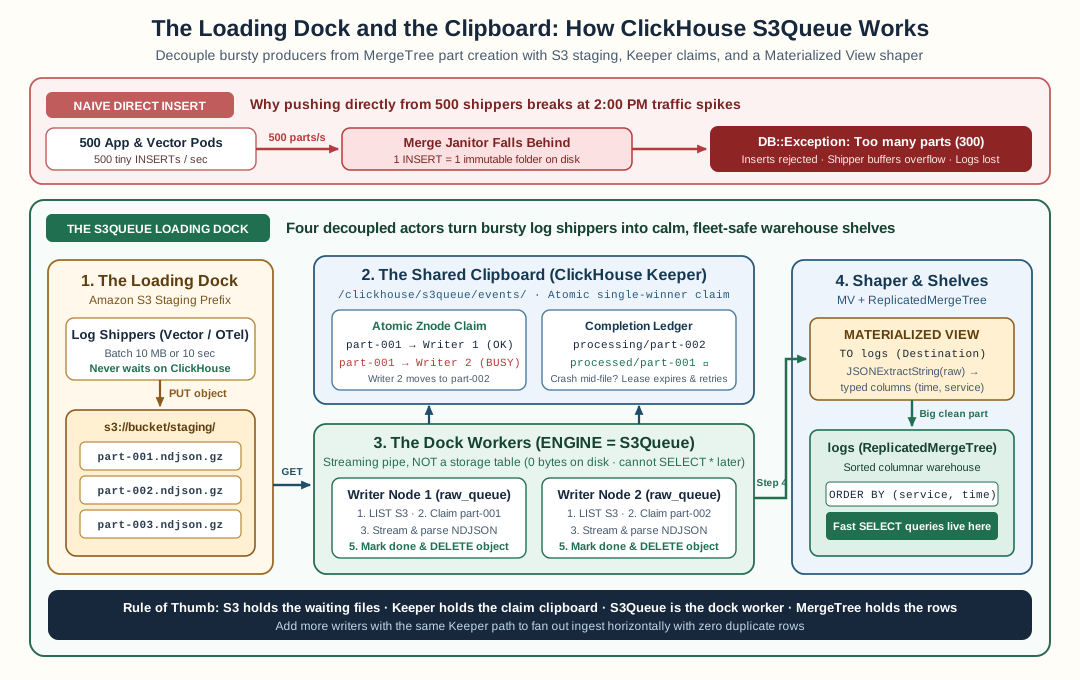
Direct inserts tie producer bursts to MergeTree part creation; the S3Queue pattern decouples them into a loading dock (S3), a shared clipboard (Keeper), streaming dock workers (S3Queue), and a shaper (Materialized View).
Step 1: the naive architecture, and the day it stops working
Start from the design everyone writes first, because it’s the design that explains the problem:
flowchart LR
    p1["Producer A"] -- INSERT --> ch[ClickHouse]
    p2["Producer B"] -- INSERT --> ch
    p3["Producer C<br/>(burst!)"] -- INSERT --> ch
Producers INSERT directly. It works on day one. Then three things happen, one per failure mode:
Failure mode 1: database-side backpressure becomes the producers’ problem. ClickHouse throttles inserts when a partition has too many unmerged parts (you know this from the MergeTree model — parts pile up faster than the background janitor can fold them). During a merge backlog or a restart, direct inserts slow down or fail. Now every producer needs retry logic, every team’s dashboard shows errors during your database’s bad afternoon, and the blast radius of database health is the whole producer fleet.
Failure mode 2: bursts couple through. One team ships a loop that inserts row-by-row. Parts explode, the throttle trips, and — because the throttle is per-partition — everyone inserting into that partition slows down. One producer’s bug is every producer’s incident.
Failure mode 3: a failed batch is gone. A direct insert that fails mid-flight has to be retried by the producer, from its own buffer, with its own bookkeeping. Producers are bad at this. “Did it commit? Half of it? Retry the whole batch or just the failed rows?” is a distributed-systems question you’ve now delegated to whichever service logs fastest.
The SQL-person summary: direct inserts are synchronous remote procedure calls into your database’s health. Staging files is an asynchronous queue with S3 as the buffer — and S3 is a spectacularly durable buffer.
Step 2: the staging pattern (the loading dock)
The fix decouples producer from consumer with one move:
flowchart LR
    subgraph producers ["Producers (any pace, any burst)"]
        p1["Producer A"]
        p2["Producer B"]
    end
    p1 -- "PUT file (NDJSON, Parquet...)" --> s3["S3 staging prefix<br/>the loading dock"]
    p2 -- "PUT file" --> s3
    s3 -- "drained at the DB's own pace" --> q["S3Queue table<br/>the dock worker"]
    q -- "parse + insert" --> t["MergeTree table<br/>the shelves"]
Producers write whole files — NDJSON, CSV, Parquet, whatever the
format — to a prefix like s3://bucket/staging/2026/11/. A PUT is a
single atomic operation: it either landed or it didn’t, and if it
didn’t the producer just… puts it again. A failed batch isn’t a lost
batch; it’s a file that’s still sitting there.
For the Postgres-minded: this is the same move as writing to a queue table or an outbox that a background worker drains — the transactional outbox pattern’s cousin — except the “outbox” is an entire S3 bucket, which means it holds any volume forever, costs cents when idle, and survives the database being rebuilt.
The trade: files that land but haven’t been read are invisible to queries. The dock has a pile; the shelves don’t know about it yet. So the pattern needs a worker — something that reads the pile, shelves the contents, and tracks what’s been done. That worker is the queue table.
Step 3: the queue table — a mailbox you can SELECT from
Here’s the engine in one CREATE:
CREATE TABLE staging_events
(
    timestamp String,
    service   String,
    message   String
    -- ...raw file columns, string-typed: the queue parses, it
    -- doesn't validate. Shaping happens in the view (step 5).
)
ENGINE = S3Queue(
    'https://bucket.s3.us-west-2.amazonaws.com/staging/*',
    'NDJSON',
    'auto'          -- the credentials mode: use the node's IAM role
)
SETTINGS
    mode = 'unordered',
    after_processing = 'delete';
From SQL’s point of view, this is a table: SELECT count() FROM
staging_events works — it reads whatever files the queue currently
has in view. From the pipeline’s point of view, it’s a background
worker with a checklist, continuously running a five-beat loop over
the prefix:
flowchart LR
    list["1. LIST<br/>what files exist?"] --> claim["2. CLAIM<br/>write initials on the clipboard"]
    claim --> parse["3. PARSE<br/>read the file into rows"]
    parse --> insert["4. INSERT<br/>rows go to the target table"]
    insert --> mark["5. MARK/DELETE<br/>cross it off — toss the cardboard"]
Walk one file through it, from the worker’s perspective:
- Discover. The engine lists the prefix. (Listing is the hidden cost of the whole design — S3 lists 1,000 keys at a time, and the drain posts in this series are largely about tuning this stage.)
- Claim. Before doing anything, the worker writes a marker — “staging/2026/11/file-42.ndjson is mine” — to the coordination service. This is the clipboard, and it’s the entire subject of step 4.
- Parse. The file’s bytes become rows of the queue table’s schema. Note the schema is deliberately raw: strings, mostly. The queue’s job is transport, not validation.
- Insert. The parsed rows flow to the target table — in practice through a materialized view (step 5). If this step fails, the marker makes the file come back for another attempt (or, in ordered mode, lands it in a recovery buffer).
- Finish.
after_processing = 'delete': the S3 object itself is deleted. The staging prefix stays small, listing stays cheap, and the bucket holding your queue costs about nothing — the cardboard gets tossed once the contents are shelved.
Step 4: the clipboard — claims, and why this is fleet-safe
Here’s the question that makes the clipboard necessary: what happens
when you run this same table on five nodes? All five poll the same
prefix. All five see file-42.ndjson. Without coordination, all five
parse it and insert it — five copies of every event.
The claim marker fixes it, and the mechanism is worth understanding precisely because it’s the same one ClickHouse replication uses elsewhere (see the roster, the journal, and the bookmarks for the full model):
- The coordination service (ClickHouse Keeper) is a shared tree of small records with one rule: only one writer can create a given path. Create-something-that-exists = refused, atomically.
- Before processing, a node creates
.../processed/file-42.ndjson— a marker naming that exact file. - Two nodes race: exactly one create succeeds. The loser sees the marker exists, shrugs, and moves to the next file.
ELI5: five dock workers share one clipboard hung by the door. Before picking up a box, a worker writes her initials and the box’s number on it. Two workers reach for the same box: the one whose pen touched paper first has it written down; the other sees the initials and picks a different box. Nobody talks to anybody; the clipboard is the conversation.
That single atomic-create rule is why the fan-out post could fix a one-node bottleneck by simply creating the same table on every writer — the fleet shares the ingest by construction, with no coordinator process, no lock service, nothing to deploy but the DDL. It’s also the exact mechanism behind the modes:
- Unordered mode (the common choice for logs): every file is independent; the marker is the dedup record. Any node, any order, maximum concurrency. If a file fails, only that file retries.
- Ordered mode: files must be processed in name order — like a queue where parcel #6 waits for #5 — for pipelines where later files carry deltas on earlier ones. The price is sequencing overhead and a dedicated recovery path for failed files.
And after_processing is the other half of the ledger:
'delete' removes the file from S3 when done (the usual choice —
staging is garbage once consumed), while 'keep' leaves it in place
and trusts the marker forever (which makes the prefix listing grow —
one of several reasons ‘delete’ is the default idiom for staging
prefixes).
One operational note that will save you an afternoon: the markers are
state. Rebuild the coordination service from scratch (or point a
fresh cluster at an old prefix) and the clipboard is blank — with
'delete', consumed files are long gone and nothing re-reads; with
'keep', everything re-reads. Neither is wrong, but you should know
which contract you chose.
Step 5: the pair — queue table + materialized view
Notice step 3’s schema was all strings. Where do DateTime columns,
generated IDs, and parsed attributes come from? From the other half
of the idiom — a materialized view:
CREATE MATERIALIZED VIEW events_shaper TO events AS
SELECT
    parseDateTime64BestEffortOrZero(timestamp, 9) AS timestamp,
    service,
    JSONExtract(message, 'status') AS status
    -- ...the shaping lives HERE, not in the queue table
FROM staging_events;
The view selects from the queue table and writes into the real MergeTree table. The division of labor is clean and worth stating because it’s the difference between a debuggable pipeline and a mystery:
- The queue table owns the file lifecycle — discover, claim, parse, delete. It never sees your business logic.
- The view owns the data shaping — types, parsing, enrichment. It never sees S3.
When a file lands wrong, you query the queue table (SELECT from it —
it’s a table!). When a row lands wrong, you fix the view. Two jobs,
two objects, no overlap — which is exactly why both drain posts could
tune one half without touching the other.
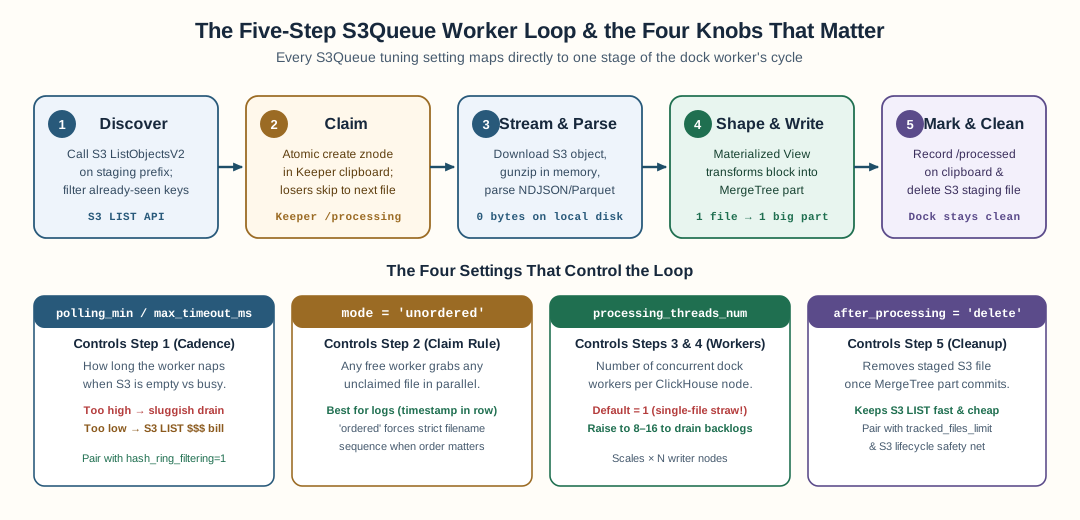
Each S3Queue tuning knob maps to one stage of the dock worker’s five-step cycle: discovery cadence, claim ordering, worker thread count, and post-processing cleanup.
When not to reach for this
The pattern costs complexity, so it should buy something real. Skip the staging prefix when:
- Volume is modest and steady. Direct batched inserts (or asynchronous inserts, which buffer server-side) are simpler and entirely healthy at the right scale.
- You need query-fresh data in seconds. The dock adds the poll-and-claim interval between “file landed” and “rows queryable.” A pipeline measured in seconds of freshness is fighting the design.
- You already run a real streaming system well. Kafka (and friends) give you ordering and replay guarantees with their own operational weight; adding an S3 dock on top of a working stream is duplication.
Reach for it when producers outnumber and out-burst your database’s comfort zone, when “the file is the record” (audit logs, export pipelines, third-party dumps), or when you want the buffer to be cheap, effectively infinite, and impossible to lose.
Now read the war stories again
With the dock, the worker, and the clipboard in hand:
- Draining 29,000 S3Queue files fast is step 1 and step 3 of the loop — discovery cadence and claim concurrency — when the pile gets big enough that the worker’s own checklist pace, not the warehouse’s, is the bottleneck.
- S3Queue is a multi-node engine is step 2 — the clipboard — proving that “deploy the same table everywhere” is not just safe but the design’s intended scaling story.
Both posts were tuning manuals for a machine this one never introduced. If you read them before and bounced off, this was the missing page.
The one-sentence model: stage the trucks on the dock (S3), let the worker with the clipboard (the queue table, claiming through Keeper) shelve boxes at the warehouse’s own pace — and the clipboard makes it safe to hire as many workers as you like.
FAQ
Why stage log files in S3 instead of inserting them into ClickHouse directly?
Decoupling. Direct inserts couple the producers' fate to the database's moment-to-moment health: a merge backlog or a restart makes inserts fail or slow, every producer needs retry logic, and a burst from one team throttles everyone. Staging files in S3 turns the database into a background consumer of a durable buffer: producers write files and move on (a failed batch is just a file that's still there), and ClickHouse drains the prefix at whatever pace its merges, disks, and replica health allow. The producers never feel database backpressure, and the database never sees producer bursts.
What is an S3Queue table?
A table whose rows live in the files of an S3 prefix instead of on local disk. The engine continuously lists the prefix, and for each file it hasn't consumed: claims it through the coordination service (Keeper), parses it, inserts the parsed rows into a target table (usually via a materialized view), and then marks or deletes the file. From SQL's point of view it behaves like a table you can SELECT from; from the pipeline's point of view it behaves like a background worker with a checklist.
What does 'claiming a file' mean, and why is there a clipboard?
Before a node processes a file, it writes a marker in Keeper — a small record in a shared tree that every node can see — saying 'file X is mine.' The write is atomic: only one node can create the marker, so two nodes racing for the same file can't both win. The marker tree is the clipboard. This is what makes the same queue table safe to deploy on many nodes: they all poll the same prefix, each file gets claimed exactly once, and the fleet shares ingest work with no coordinator process.
What is the difference between unordered and ordered mode?
Ordered mode processes files in the strict order they appear (by name), like a queue where you must finish parcel #5 before opening #6 — useful when later files depend on earlier ones, and it pays for that with coordination overhead and a recovery buffer for failed files. Unordered mode processes any claimed file at any time and tracks each consumed file by name in a Keeper record, deduplicating by marker rather than by sequence — the common choice for log files, where every file is independent and throughput is the point.
What does after_processing = 'delete' do?
It is the cleanup philosophy of the queue: after a file's rows are committed, delete the S3 object. The alternative, 'keep', leaves the file in place and relies on the Keeper marker to skip it forever. Delete is the usual choice for a staging prefix — consumed files are garbage, and deleting them keeps both the S3 listing small and the cost near zero — but it means re-processing a file after a wipe (a rebuilt Keeper, a fresh cluster pointed at the same prefix) has nothing left to read.
How does the queue table connect to the target table?
Usually through a materialized view. The queue table parses files into raw staging rows; a materialized view SELECTs from the queue table and inserts transformed rows (parsed timestamps, generated IDs, mapped columns) into the real MergeTree table. The pair — staging queue plus transformation view — is the idiom: the queue handles the file lifecycle, the view handles the data shaping, and neither job contaminates the other.
Stay in the loop — production notes on AI agents, workflows, and SRE.
Low volume — new posts and curated reading lists. Unsubscribe anytime.